Date-Time Cycling¶

In the last section we looked at writing an integer cycling workflow, one where the cycle points are numbered.

Typically workflows are repeated at a regular time interval, say every day or every few hours. To make this easier Cylc has a date-time cycling mode where the cycle points use date and time specifications rather than numbers.

Reminder

Cycle points are labels. Cylc runs tasks as soon as their dependencies are met so cycles do not necessarily run in order.

ISO8601¶

In Cylc, dates, times and durations are written using the ISO8601 format - an international standard for representing dates and times.

Date-Times¶

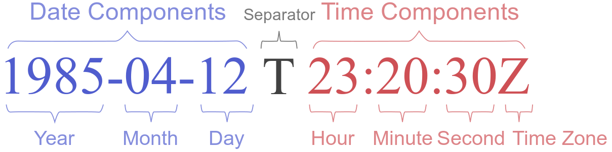
In ISO8601, datetimes are written from the largest unit to the smallest (i.e: year, month, day, hour, minute, second in succession) with the T character separating the date and time components. For example, midnight on the 1st of January 2000 is written 20000101T000000.

For brevity we may omit seconds (and minutes) from the time i.e: 20000101T0000 (20000101T00).

For readability we may add hyphen (-) characters between the date components and colon (:) characters between the time components, i.e: 2000-01-01T00:00. This is the “extended” format.

Time-zone information can be added onto the end. UTC is written Z, UTC+1 is written +01, etc. E.G: 2000-01-01T00:00Z.

Warning

The “basic” (purely numeric except for T) and “extended” (written with hyphens and colons) formats cannot be mixed. For example the following date-times are invalid:

2000-01-01T0000
20000101T00:00

Durations¶

In ISO8601, durations are prefixed with a P and are written with a character following each unit:

Y for year.
M for month.
D for day.
W for week.
H for hour.
M for minute.
S for second.

As with datetimes the components are written in order from largest to smallest and the date and time components are separated by the T character. E.G:

P1D: one day.
PT1H: one hour.
P1DT1H: one day and one hour.
PT1H30M: one and a half hours.
P1Y1M1DT1H1M1S: a year and a month and a day and an hour and a minute and a second.

Date-Time Recurrences¶

In integer cycling, suites’ recurrences are written P1, P2, etc.

In date-time cycling there are two ways to write recurrences:

Using ISO8601 durations (e.g. P1D, PT1H).
Using ISO8601 date-times with inferred recurrence.

Inferred Recurrence¶

A recurrence can be inferred from a date-time by omitting digits from the front. For example, if the year is omitted then the recurrence can be inferred to be annual. E.G:

2000-01-01T00   # Datetime - midnight on the 1st of January 2000.

     01-01T00   # Every year on the 1st of January.
        01T00   # Every month on the first of the month.
          T00   # Every day at midnight.
          T-00  # Every hour at zero minutes past (every hour on the hour).

Note

To omit hours from a date time we must place a - after the T character.

Recurrence Formats¶

As with integer cycling, recurrences start, by default, at the initial cycle point. We can override this in one of two ways:

By defining an arbitrary cycle point (datetime/recurrence):
- 2000/P1Y: every year starting with the year 2000.
- 2000-01-01T00/T00: every day at midnight starting on the 1st of January 2000
- 2000-01-01T12/T00: every day at midnight starting on the first midnight after the 1st of January at 12:00 (i.e. 2000-01-02T00).

By defining an offset from the initial cycle point (offset/recurrence). This offset is an ISO8601 duration preceded by a plus character:
- +P1Y/P1Y: every year starting one year after the initial cycle point.
- +PT1H/T00: every day starting on the first midnight after the point one hour after the initial cycle point.

Durations And The Initial Cycle Point¶

When using durations, beware that a change in the initial cycle point might produce different results for the recurrences.

[scheduling]
    initial cycle point = 2000-01-01T00
    [[dependencies]]
        [[[P1D]]]
            graph = foo[-P1D] => foo

[scheduling]
    initial cycle point = 2000-01-01T12
    [[dependencies]]
        [[[P1D]]]
            graph = foo[-P1D] => foo

We could write the recurrence “every midnight” independent from the initial cycle point by:

Use an inferred recurrence instead (i.e. T00).
Overriding the recurrence start point (i.e. T00/P1D)
Using the [scheduling]initial cycle point constraints setting to constrain the initial cycle point (e.g. to a particular time of day). See the Cylc User Guide for details.

The Initial & Final Cycle Points¶

There are two special recurrences for the initial and final cycle points:

R1: repeat once at the initial cycle point.
R1/P0Y: repeat once at the final cycle point.

Inter-Cycle Dependencies¶

Inter-cycle dependencies are written as ISO8601 durations, e.g:

foo[-P1D]: the task foo from the cycle one day before.
bar[-PT1H30M]: the task bar from the cycle 1 hour 30 minutes before.

The initial cycle point can be referenced using a caret character ^, e.g:

baz[^]: the task baz from the initial cycle point.

UTC Mode¶

Due to all of the difficulties caused by time zones, particularly with respect to daylight savings, we typically use UTC (that’s the +00 time zone) in Cylc suites.

When a suite uses UTC all of the cycle points will be written in the +00 time zone.

To make your suite use UTC set the [cylc]UTC mode setting to True, i.e:

[cylc]
    UTC mode = True

Putting It All Together¶

Cylc was originally developed for running operational weather forecasting. In this section we will outline a basic (dummy) weather-forecasting suite and explain how to implement it in cylc.

Note

Technically the suite outlined in this section is a nowcasting suite. We will refer to it as forecasting for simplicity.

A basic weather-forecasting workflow consists of three main steps:

1. Gathering Observations¶

We gather observations from different weather stations and use them to build a picture of the current weather. Our dummy weather forecast will get wind observations from four weather stations:

Aldergrove
Camborne
Heathrow
Shetland

The tasks which retrieve observation data will be called get_observations_<site> where site is the name of the weather station in question.

Next we need to consolidate these observations so that our forecasting system can work with them. To do this we have a consolidate_observations task.

We will fetch wind observations every three hours starting from the initial cycle point.

The consolidate_observations task must run after the get_observations<site> tasks.

We will also use the UK radar network to get rainfall data with a task called get_rainfall.

We will fetch rainfall data every six hours starting six hours after the initial cycle point.

2. Running computer models to generate forecast data¶

We will do this with a task called forecast which will run every six hours starting six hours after the initial cycle point. The forecast task will be dependent on:

The consolidate_observations task from the previous two cycles as well as from the present cycle.
The get_rainfall task from the present cycle.

3. Processing the data output to produce user-friendly forecasts¶

This will be done with a task called post_process_<location> where location is the place we want to generate the forecast for. For the moment we will use Exeter.

The post_process_exeter task will run every six hours starting six hours after the initial cycle point and will be dependent on the forecast task.

Practical

In this practical we will create a dummy forecasting suite using date-time cycling.

Create A New Suite.

Within your ~/cylc-run directory create a new directory called datetime-cycling and move into it:

mkdir ~/cylc-run/datetime-cycling
cd ~/cylc-run/datetime-cycling

Create a suite.rc file and paste the following code into it:

[cylc]
    UTC mode = True
[scheduling]
    initial cycle point = 20000101T00Z
    [[dependencies]]

Add The Recurrences.

The weather-forecasting suite will require two recurrences. Add sections under the dependencies section for these, based on the information given above.

Hint

See Date-Time Recurrences.
Solution

The two recurrences you need are
- PT3H: repeat every three hours starting from the initial cycle point.
- +PT6H/PT6H: repeat every six hours starting six hours after the initial cycle point.
```
 [cylc]
     UTC mode = True
 [scheduling]
     initial cycle point = 20000101T00Z
     [[dependencies]]
+        [[[PT3H]]]
+        [[[+PT6H/PT6H]]]
```

Write The Graphing.

With the help of the graphs and the information above add dependencies to your suite to implement the weather-forecasting workflow.

You will need to consider the inter-cycle dependencies between tasks.

Use cylc graph to inspect your work.

Hint

The dependencies you will need to formulate are as follows:

The consolidate_observations task is dependent on the get_observations_<site> tasks.
The forecast task is dependent on:
- the get_rainfall task;
- the consolidate_observations tasks from:
  - the same cycle;
  - the cycle 3 hours before (-PT3H);
  - the cycle 6 hours before (-PT6H).
The post_process_exeter task is dependent on the forecast task.

To launch cylc graph run the command:

cylc graph <path/to/suite.rc>

Solution

[cylc]
    UTC mode = True
[scheduling]
    initial cycle point = 20000101T00Z
    [[dependencies]]
        [[[PT3H]]]
            graph = """
                get_observations_aldergrove => consolidate_observations
                get_observations_camborne => consolidate_observations
                get_observations_heathrow => consolidate_observations
                get_observations_shetland => consolidate_observations
            """
        [[[+PT6H/PT6H]]]
            graph = """
                consolidate_observations => forecast
                consolidate_observations[-PT3H] => forecast
                consolidate_observations[-PT6H] => forecast
                get_rainfall => forecast => post_process_exeter
            """

Inter-Cycle Offsets.

To ensure the forecast tasks for different cycles run in order the forecast task will also need to be dependent on the previous run of forecast.

We can express this dependency as forecast[-PT6H] => forecast.

Try adding this line to your suite then visualising it with cylc graph.

You will notice that there is a dependency which looks like this:

Note in particular that the forecast task in the 00:00 cycle is grey. The reason for this is that this task does not exist. Remember the forecast task runs every six hours starting 6 hours after the initial cycle point, so the dependency is only valid from 12:00 onwards. To fix the problem we must add a new dependency section which repeats every six hours starting 12 hours after the initial cycle point.

Make the following changes to your suite and the grey task should disappear:
```
           [[[+PT6H/PT6H]]]
               graph = """
                   ...
-                  forecast[-PT6H] => forecast
               """
+          [[[+PT12H/PT6H]]]
+              graph = """
+                  forecast[-PT6H] => forecast
+              """
```